Tensorflow 2: NLP for Netflix Data
Environment
Python 3.6 with: Tensorflow (v2.1), Sklearn, Pandas, Matplotlib, Numpy, Datetime
All development for this project was done within Google Colab notebooks. This choice was made for a few reasons:
- Colab notebooks provide hardware acceleration for free. I don’t have a PC that is supported with Tensorflow hardware acceleration, so Colab saved significant runtime.
- Sharing my work in Colab is very easy.
- Using Colab gave me more experience with it. While I had plenty of experience with Jupyter notebooks, I had only used Colab for my Coursera classes on Tensorflow.
Links to my Colab notebooks will are provided in the Modeling section below.
Introduction
The goal of this project was to get my hands dirty using Tensorflow, having recently completed Coursera courses on Tensorflow 2. I decided to focus on an NLP (natural language processing) project, ultimately selecting a common Kaggle dataset with the goal of predicting the genres of movies and TV shows based on their descriptions. Since multiple genres are permitted for each item, this is a multi-label classification problem. Regarding modeling, I wanted to experiment with building my own complete neural network from scratch and compare it with a popular pre-trained NLP model named BERT.
Data
This project uses a common Kaggle dataset: Netflix Movies and TV Shows (Version 3). The csv file contains data for movie and TV show items that were available on Netflix in 2019. The fields utilized in this project are listed_in and description. listed_in provides the genres under which the item was categorized. There are 42 possible genres, and each item may have multiple genres assigned to it. description is a free text field which describes the basic storyline of the of the item. In total there are 6,234 items in the dataset.
This data was read into a Pandas dataframe and the two aforementioned fields were isolated. The data was reshaped into a new dataframe which resembling a one-hot-encoder array, where each column represents whether a genre was assigned to each item. Lastly, this dataframe was converted into a Tensorflow tensor and split into training and test tensors, with 80% of the rows being assigned to the training tensor.
Modeling
Custom Neural Network
The first modeling approach to this project was to construct a neural network from scratch. This began with tokenizing the description text, which converted the text into a list of arbitrary integers (each integer representing a word). The neural networks used here will not accommodate batched inputs of varying length, so each tensor element in each batch was padded to make all elements equal in length to th longest batch element.
The next step was to define the neural network architecture. The fundamental architecture consisted of an embedding layer as its input, recurrent network layers as the hidden layers and the output layer as a fully connected dense layer. The embedding input layer had as many nodes as the vocabulary size in the training data set, with an additional node for out-of-vocabulary words that might only be in the test data set. The dense output layer had 42 nodes with a sigmoid activation function to provide a liklihood for each genre option.
Many architectures were tried utilizing simple recurrent layers, LSTMs and bi-directional LSTMs. Dropout layers were also added for regularization and the number of dense layers at the top of the network was varied. In addition, the parameters of these layers were varied, including the number of dimensions to embed the vocabulary in and the width of the layers. The following model summary shows the architecture of the final model.
Model: "sequential_1"
_________________________________________________________________
Layer (type)                 Output Shape              Param #
=================================================================
embedding_1 (Embedding)      (None, None, 8)           6824
_________________________________________________________________
bidirectional_2 (Bidirection (None, None, 64)          10496
_________________________________________________________________
bidirectional_3 (Bidirection (None, 64)                24832
_________________________________________________________________
dense_2 (Dense)              (None, 32)                2080
_________________________________________________________________
dropout_1 (Dropout)          (None, 32)                0
_________________________________________________________________
dense_3 (Dense)              (None, 42)                1386
=================================================================
Total params: 45,618
Trainable params: 45,618
Non-trainable params: 0
_________________________________________________________________
These models were trained using the ADAM optimizer and a custom loss function found here. Typically binary cross-entropy is used in classification problems, then the threshold for each label is chosen with a validation data set. The results would then be evaluated using the F1 score metric, which is not differentiable and therefore can’t be used as the loss function. The custom loss function provides a better measure of loss for multi-label classification problems by enabling the F1 score to be used as the loss function, thereby avoiding the task of setting thresholds. This is done by supplying the F1 score formula with the predicted likelihood as opposed to binary values obtained through thresholding. This is called a soft F1 score.
BERT Pre-trained Network
BERT is a collection of deep language models trained by Google on vast corpora. In this project, a BERT model was used that was trained on English articles in lowercase with 128 embedding dimensions. Two dense layers were appended on top of the BERT pre-trained network. The output layer in this model is identical to the one used in the custom NN. The only architecture tuning was performed on the dense hidden layer(s) connecting the BERT model to the output layer. The same optimization and loss functions were used in these models as in the custom NN. The following model summary shows the architecture of the final model.
Model: "sequential"
_________________________________________________________________
Layer (type)                 Output Shape              Param #
=================================================================
keras_layer (KerasLayer)     (None, 128)               124642688
_________________________________________________________________
dense (Dense)                (None, 64)                8256
_________________________________________________________________
dense_1 (Dense)              (None, 42)                2730
=================================================================
Total params: 124,653,674
Trainable params: 10,986
Non-trainable params: 124,642,688
_________________________________________________________________
Results
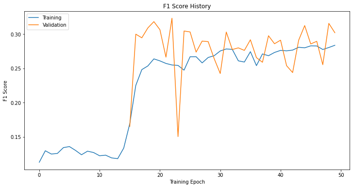
Not surprisingly, the BERT model crushed the custom NN model. The figure below plots the F1 scores on the training and validation datasets during training. The maximum F1 score on the validation data set was 0.323. The figure suggests that model isn’t training well because the validation score peaks early in the training history and makes significant oscillations afterwards. A model that is training well will smoothly and monotonically maximize the evaluation metric.

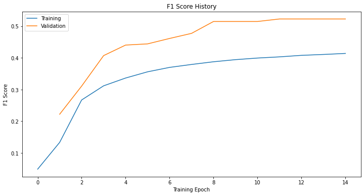
The figure below plots the same metric history when training the dense layers appended on top of the BERT model. The maximum F1 score on the validation data set was 0.523, far exceeding the 0.323 score mentioned above. The figure also illustrates how a model that is training well will smoothly improve its evaluation metric.


