Supervised ML: Don’t Overfit! II

Environment

Python 3.7 with: Sklearn, Matplotlib, Seaborn, Graphviz, Vecstack, Pandas, Numpy, Scipy, Random, os, itertools

A conda environment for data science was created, and all of the programming was implemented in a Jupyter notebook. All of the associated files have been placed in my project repository on Github, and the README.md file provides instructions for reproducing my results.

Introduction

The goal of this Kaggle competition was to predict the binary classification of 19,750 observations given data for 250 observations and 300 features. My interest in this project was to develop more broad experience with various machine learning classifier models.

Findings

Fourteen models were generated in this analysis, six of which were ensembles based on eight base models. The ensemble techniques provided only a small improvement on the best base models. Models were evaluated using the metric ROC AUC because this is the metric used to score submissions. Most of the models have their ROC curve plotted below. ROC is a curve which represents how often a model predicts false positives (X-axis) and true positives (Y-axis) as the threshold for classification is altered. Hence it can rank various models independent of threshold. ROC AUC is the measure of Area Under Curve of the ROC curve. The greater AUC is, the better the model is at distinguishing beteen false positives and true positives.

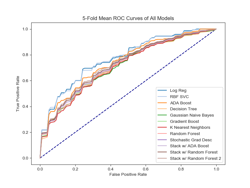
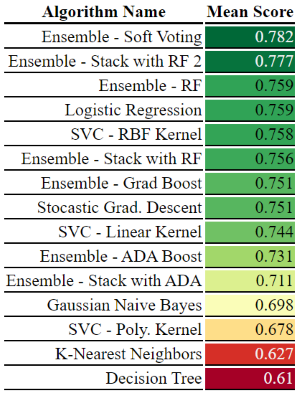
The following table gives the 5-fold mean ROC AUC score for every model created in this analysis. Most of these models were hypertuned using GridSearchCV. The most surprising result in this analysis was that Logistic Regression nearly matches the best ensemble, despite the fact that it wasn’t hypertuned.

Methodology Highlights

Data Cleaning

No missing values exist in the datasets provided. All feature data is continuous and is already standardized. Therefore no cleaning was required.

Exploratory Data Analysis

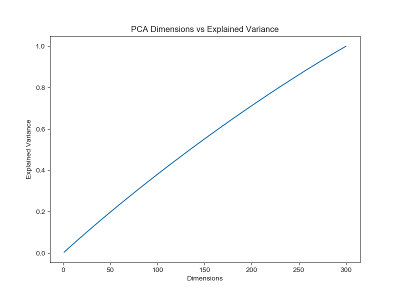
First, the data was explored with the aim of feature reduction. Principal Component Analysis (PCA) was used to discern some features were more important than others. The plot below indicates that all features have equal importance because the plot forms a straight line. If some features were more important, then the line would resemble a monotonically decreasing function (concave down).

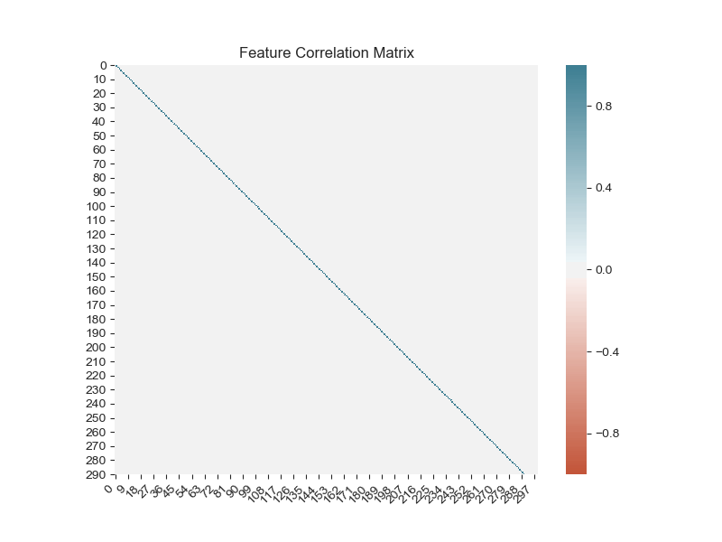
The feature correlations matrix is also plotted below. Note, since PCA had indicated that all features were equally important, this correlation plot was expected to show all features to be independent. Since no correlations were found between features, no features were eliminated in subsequent analysis.

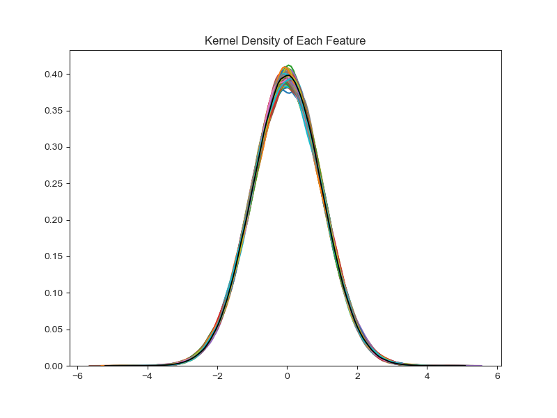
Kernel density plots were also overlaid for all 300 features. The underlying feature data utilizes both training and test datasets. In addition, the mean and standard deviation were derived from the entire feature population and the resulting normal distribution was plotted in black. This shows that all features are approximately Gaussian. Taken alongside the PCA results, the strong similarity in feature distributions suggests the features are independent and identically distributed (iid).

Modeling

The following eight base models were created (bold font indicates the model was hypertuned): Logistic Regression, Support Vector Classification (SVC) with a linear kernel, SVC with a polynomial kernel, SVC with a radial basis function kernel, K-Nearest Neighbors, Decision Tree, Stochastic Gradient Descent and Gaussian Naive Bayes. All models were cross validated with 5-folds and scored based on the 5-fold mean ROC AUC score.

Next, six ensemble models were constructed and all were hypertuned: Random Forest, ADA Boost based on Decision Tree models, Gradient Boost, Soft Voting based on 9 models, ADA Boost Stacked on top of 9 models, Random Forest stacked on top of 9 models, Random Forest stacked on the 3 most important models from the aforementioned set of 9. These models were also cross validated with 5-folds and scored based on the 5-fold mean ROC AUC score.

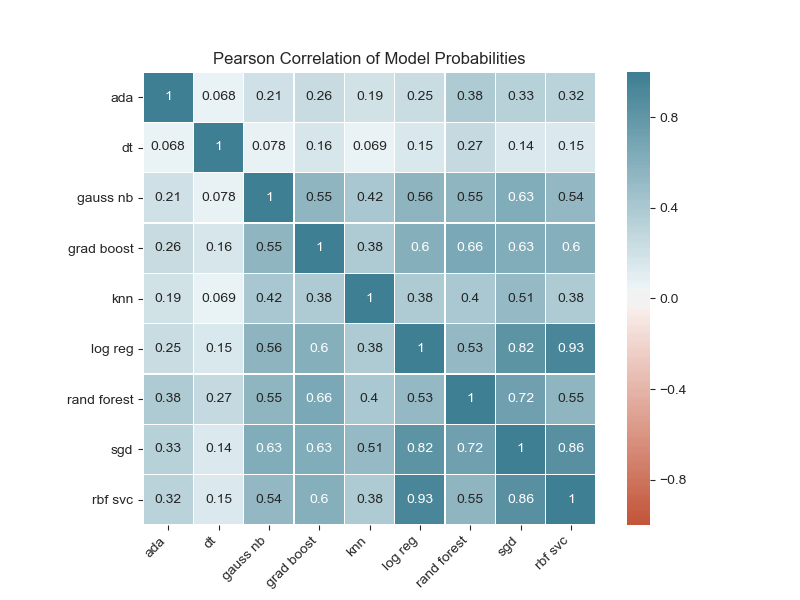
Prior to building ensembles which relied on extant base models, the base models were checked for whether their predicted probabilities were correlated. The plot shows that most models do not have strong correlation (< 0.8).

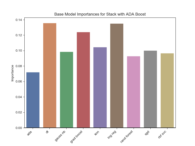
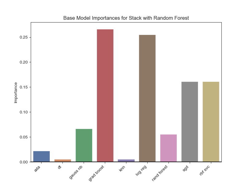
Lastly, after the stacked models were completed, feature importance was plotted to determine which base models were most important. The plots below give the base model importance when ADA Boost and Random Forest is stacked on top. Since Random Forest depended heavily on three base models, a similar model was created which only relied on those three most important models. This last model is named “Ensemble - Stack with RF 2” in the model score table above. It slightly improved the performance of its predecessor.

What Could Be Improved?

Reading some of the notebooks and discussion threads on the Kaggle competition website, feature importance was examined using partial dependence, the ELI5 package and the SHAP package. All of these are defined in this Kaggle notebook. In addition, when tuning ensemble models, recursive feature elimination (RFE) could have been utilized to accomplish more extensive tuning.

Also, alternate metrics could be added to the model evaluation. The Wikipedia page for ROC mentions that ROC AUC has a few shortcomings: it can be noisy, it ignores performance in specific threshold regions and only half of the measure is useful (<0.5 means it is worse than a random selection). Alternative metrics are: Informedness, Markedness, Matthews correlation coefficient, Certainty, Gini coefficient and Total Operating Characteristic.

And lastly, evaluating distances between observations in hyperspace can be a good method of identifying patterns in target behavior. While K nearest relies on euclidean distance, other measures of distance could be considered.